Finite Cell Method

Overview:

The Finite Element Method (FEM) is the standard tool to solve problems of computational mechanics in complex domains. Thereby, the essential step of the simulation process is the discretization of the physical domain yielding a FE mesh. This task, however, can be very challenging and time consuming, especially for complex real life applications.

To overcome this problem, the chair of Computation in Engineering (CiE) has developed the Finite Cell Method (FCM) which does not capture the complexity of the geometry on the mesh- but on the integration-level. Recent research shows excellent applicability of this new idea in the fields of linear and non-linear structural mechanics, topology optimization, thin-walled structures, bone mechanics and advection-diffusion problems.

High order finite elements:

The finite cell method utilizes higher order finite elements, which are robust against geometric distortions and lead to very accurate even for non-smooth problems. Besides the p-version of the FEM recent works have also applied B-spline and NURBS bases in the framework of the FCM.

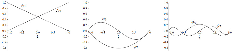
Figure 1: Linear nodal modes N_j, j=1, 2 and the first 4 integrated Legendre basis functions φ_j, j=2, ..., 5 of the 1D
p-version basis in the parameter space ξ. Their combination yields the shape functions of a 1D finite cell of p=5.¹

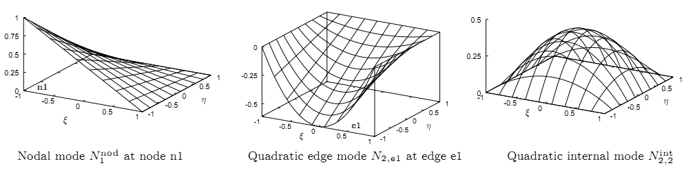
Figure 2: Examples of shape functions of the 2D p-version basis in the parameter space [ξ, η].¹

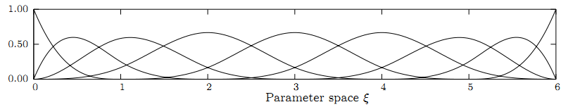
Figure 3: Example of an open cubic B-spline patch with 3 uniform B-splines and 6 knot spans.¹

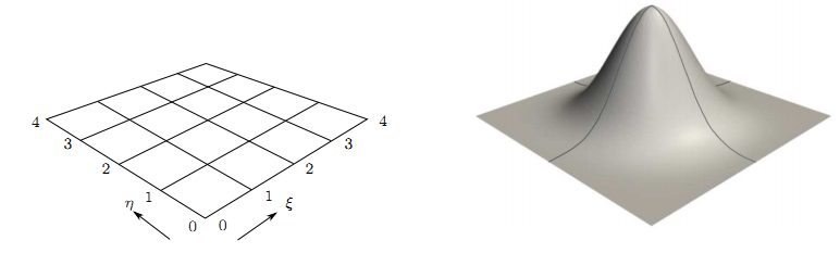
Figure 4: Knot span cells in the parameter space {ξ, η} (left) and corresponding bi-variate cubic B-spline (right).¹

Adaptive Integration: Since the FCM operates on a unfitted simple cartesian grid, the geometry has to be recovered at the integration level. Therefore an adaptive integration scheme is applied, which hierachically decomposes the cells into integration sub-cells. An example for a decomposition in 2D is shown in Fig 5.

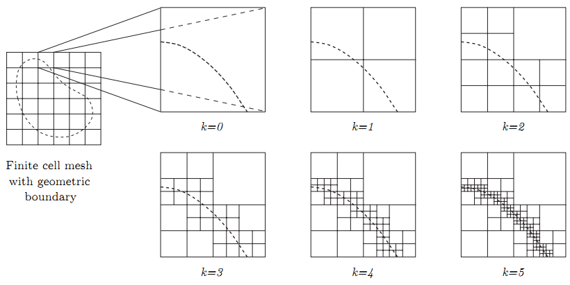
Figure 5: 2D sub-cell structure for adaptive integration of cells cut by the geometric boundary.¹