Non-destructive testing using full waveform inversion

The contract person for this project is Philipp Kopp (This email address is being protected from spambots. You need JavaScript enabled to view it.) and Stefan Kollmannsberger. Most of the work was done by Dr. Robert Seidl during his time at the chair. There will be a new initiative in this direction by the help of the DFG Grant No. KO 4570/1-1 and RA 624/29-1.

Non destructive testing (NDT):

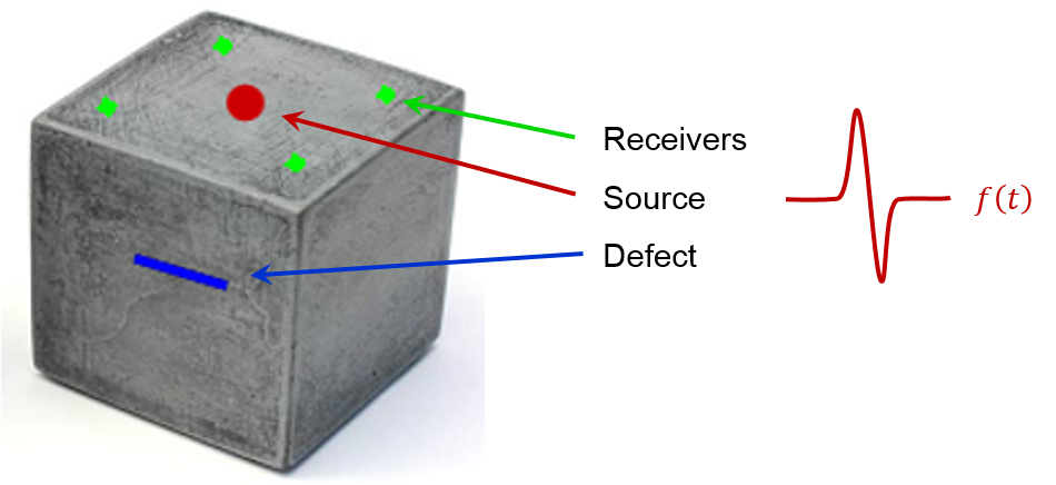
Non-destructive testing addresses the following question: How can we detect flaws in mechanical compnents without destroying them? In general, the procedure for any method in NDT is the following:

        1. Perform non-destructive experiments.

        2. Compare to measurements on intact body.

In the experiments the object is excited with an impulse and its response is measured at given receiver positions. The recorded signal is then compared to the measurements performed on an intact body. If the difference of both signals is significant, we can assume that our component is flawed. However, in practice, we might

• not have an intact component
• need geometric information about defect
• need mechanical properties of the defect.

These shortcomings are addressed by the full waveform inversion.

Full waveform inversion (FWI):

In the full waveform inversion the intact component is modelled mathematically and the mechanical resonse is simulated numerically (this is called the forward problem). We use the very simple model of an accoustic wave equation to demonstrate the concept. The goal is to tune this model such that the simulation result match the measurements of the flawed component as good as possible. In other words, we would like to find a wave speed c(x) that delivers a numerical solution u(x) that matches the measurements m(x) at the receiver positions.

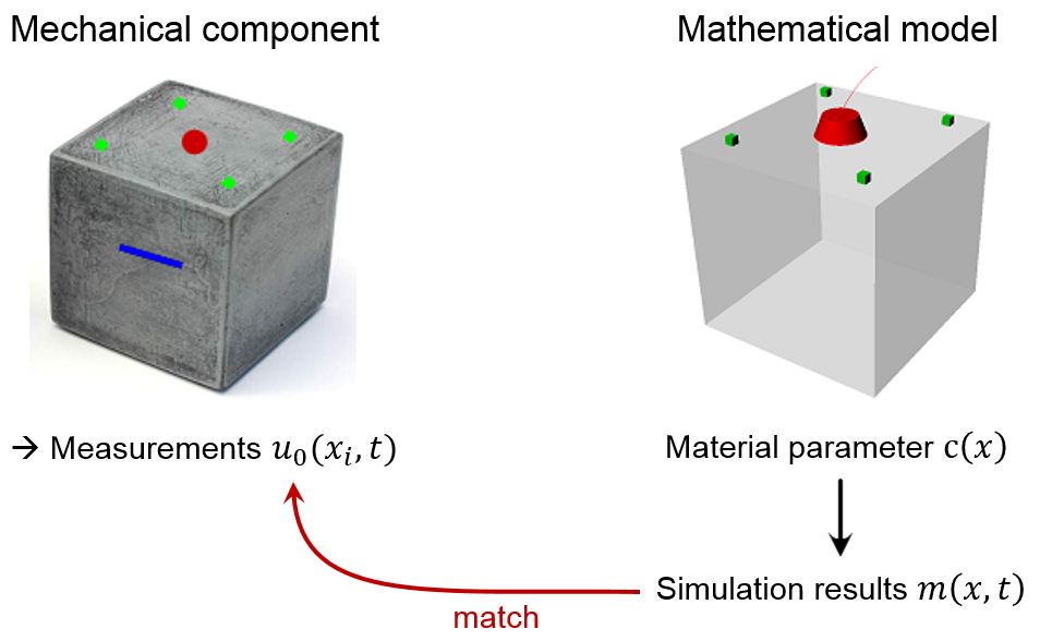
This poses an inverse problem that is formulated as follows: Find c(x) such that u(x, t) matches m(x, t) as good as possible.

From the material parameter c(x) we can deduce spatial and mechanical information about defects. This concept is valid for any model, in practice we might need to use more sophisticated mathematical models, such as linear elasticity.

The remaining piece is to specify what "matches closely" means by defining a misfit function (also called objective function) that computes the error for a given material configuration c(x). In our case we simply sum up the squares of the differences between measured and simulated signal at the receiver positions. With this step we have turned an inverse problem into a minimization problem that we can solve iteratively by, e.g., a gradient descent method.

Research:

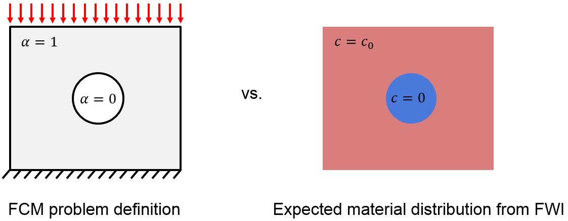
Recently, we tried to combine the full waveform inversion with the finite cell method (FCM). A straight forward combination would be to use FCM as discretization technique in the solution of the forward problem. However, another connection can be drawn by interpreting the result of the FWI, i.e. a material field incorporating the geometry of the flaw, as an FCM-like description. This is motivated as follows: To obtain an FCM description of a flawed geometry the material coefficient (e.g. a Young's modulus, or, in out case the wave speed) is multiplied by a very small value outside the pysical domain, i.e. inside a crack. The resulting material field, however, is precisely what we hope to obtain from a full waveform inversion.

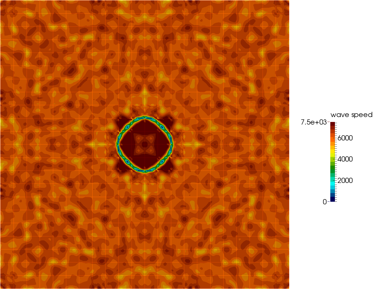
Motivated by this we considered a classical plate with a hole, where the hole is now interpreted as flaw. We generate synthetic measurements using an FCM simulation of the forward problem. We then "forget" about the hole and try to reconstruct a material field c(x) from FWI, hoping that it resembles the FCM solution we started with. The setup looks as follows:

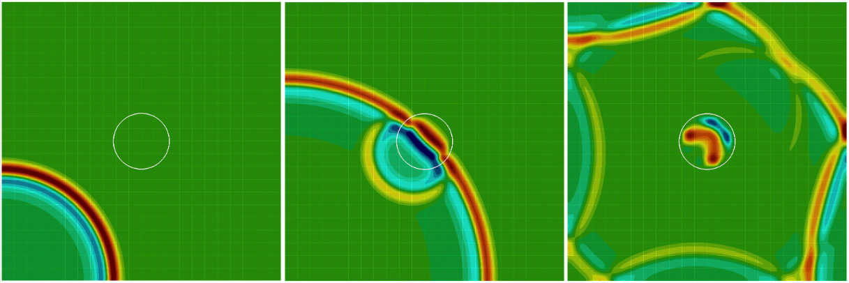
The following figure shows the generation of synthetic measurement data m(x) using FCM. The white circle represents the boundary to the fictitious disk (our flaw) in the middle.

The simulation was performed on a mesh with 22 elements in each direction and a polynomial degree of 8 (using a trunk space) giving a total of 14873 degrees of freedom.

With this data we set up an inverse problem performing 8 experiments (with a difference source each experiment) and using 16 receiver locations (receivers are green, sources are red):

The mesh is the same we used to generate the measurements. The inversion using this setup reached a local minimum after 84 gradient descent iterations, giving the following material field:

 The evolution of the misfit functional

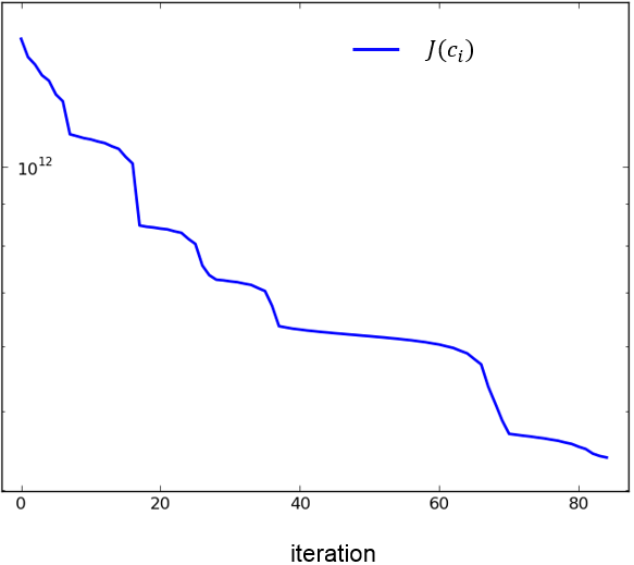
Overall the results are great, as a sharp boundary of the flaw was recovered. However, more attention has to be devoted towards the design of the objective functional, as a local minimum was reached rather quick.

Publications:

• Seidl, R.; Rank, E. Show abstract Full waveform inversion for ultrasonic flaw identification
  In: AIP Conference Proceedings 1806, 090013 (2017), , 2017
  
  
  
  Ultrasonic Nondestructive Testing is concerned with detecting flaws inside components without causing physical damage. It is possible to detect flaws using ultrasound measurements but usually no additional details about the flaw like position, dimension or orientation are available. The information about these details is hidden in the recorded experimental signals. The idea of full waveform inversion is to adapt the parameters of an initial simulation model of the undamaged specimen by minimizing the discrepancy between these simulated signals and experimentally measured signals of the flawed specimen. Flaws in the structure are characterized by a change or deterioration in the material properties. Commonly, full waveform inversion is mostly applied in seismology on a larger scale to infer mechanical properties of the earth. We propose to use acoustic full waveform inversion for structural parameters to visualize the interior of the component. The method is adapted to US NDT by combining multiple similar experiments on the test component as the typical small amount of sensors is not sufficient for a successful imaging. It is shown that the combination of simulations and multiple experiments can be used to detect flaws and their position, dimension and orientation in emulated simulation cases.
  
  
  
• Seidl, R.; Rank, E. Show abstract Iterative time reversal based flaw identification
  Computers & Mathematics with Applications 72 (4), pp. 879-892, 2016
  DOI: 10.1016/j.camwa.2016.05.036
  
  
  
  In the field of ultrasonic non-destructive testing, ultrasonic impulses are used to detect flaws in components without causing damage. Based on performing experiments alone, it is possible to infer the state of the component–but this usually provides only limited details about the interior damage such as its position, dimension or orientation. Furthermore, the amount of sensors that can be used to record the signals is restricted to only a few because of the shape and the dimensions of a typical specimen and considerations such as costs, additional mass and structural integrity. Further information about the flaw is hidden in the recorded experimental signals. The idea of the proposed method is to use the experimental data together with a wave speed model of a healthy component and to try to adapt the model to generate these experimental measurements. Formally, the problem is posed as a nonlinear optimization, and the wave speed model is adapted in such a way that the discrepancy between the experimental measurements and the model output is minimized. Moreover, to overcome the problem of only a few available sensor measurements, a combination of multiple simulations corresponding to generally performed multiple experiments in SHM practice is used to improve the accuracy. Following this approach, the position, dimension and orientation of a flaw can be detected for an emulated damaged aluminum plate. For cases when there are only few sensors available, it is shown how a combination of similar experiments can be used to improve the inversion results.